Below is the online edition of In the Beginning: Compelling Evidence for Creation and the Flood,
by Dr. Walt Brown. Copyright © Center for Scientific Creation. All rights reserved.
Click here to order the hardbound 8th edition (2008) and other materials.
Calculations That Show Comets Began Near Earth
If the most clocklike comets can be shown to have begun near Earth with a very high probability (>99%), one can also directly conclude with a high probability that:
If these conclusions are shocking to some individuals, here is their challenge: Find an error in the calculations outlined below, or seriously consider the mathematical conclusions. For more details, see "When Was the Flood, the Exodus, and Creation?" on pages 493–496.
Step 1: Download from the internet the two papers referenced in Endnote 5 on page 495.1 They are located at
http://adsabs.harvard.edu/full/1981MNRAS.197..633Y
and
http://adsabs.harvard.edu/full/1994MNRAS.266..305Y
After reading both papers, set up a workbook in Excel 2007 (or higher) with the following worksheets:
a. Most Clocklike Comets
b. True Deviations Squared
c. Random Deviations Squared
Data and calculations from worksheets a–b will feed into subsequent worksheets.
Set up a table in the “Most Clocklike Comets” worksheet similar to Table 40 and fill in all 49 rows. Some cells will require simple calculations. Select any Julian date converter on the internet and become comfortable converting from calendar dates to Julian dates and vice versa.
Step 2: Set up a table in the “True Deviations Squared” worksheet similar to Table 41. Designate a row in column B for each of the past 4,000–6,000 years. In column C, calculate the corresponding Julian dates. In columns D and E (for comets Halley and Swift-Tuttle, respectively), calculate the number of days until (or since) that comet’s nearest perihelion. Square that number, and place the sum of those two squared numbers in the corresponding row in column G. Place the minimum of the numbers in column G in cell G1 and the corresponding Julian date and calendar date in cells G2 and G3. That is the year in which the three bodies (Halley, Swift-Tuttle, and Earth) were closest to each other. However, the degree of closeness may not be statistically significant. That significance will be determined in Step 3. Plot column G vs. column B (time), as shown in Figure 254.
Excel spreadsheets have built in functions that can save you a great deal of time. Consider using the functions: SQRT (square root), STDEV (sample standard deviation), MIN (minimum), and RAND (random number). Also macros can repeat complex operations in milliseconds.
Step 3: In the “Random Deviations Squared” worksheet, repeat Step 2, but begin each comet’s backward march from a random point on its oldest known orbit instead of its perihelion. With a macro, repeat this process 1,000,000 times (for the time interval 4,000–6,000 years ago) and see what percent of those random trials produced a clustering at least as tight as you got in Step 2. Your answer should be only about 0.6 of 1%. Alternatively, if we began each comet’s backward projection from a random point on its oldest known orbit, we would have to search 333,333 years, on average, to find one clustering that was at least as tight. [2,000/(0.006)= 333,333]
Step 4: Calculate the expected error for each comet individually. Those errors can be determined by three different methods: A, B, and C. All give the same answer. Method A, a simple, intuitive approach, will now be explained using comet Halley as an example.
Method A: Geometric. Visualize a timeline extending back in time from Halley’s oldest known perihelion in 1403.80 B.C. If we tick off exactly 27 69.86-year increments on that timeline, we will be at 3290 B.C.—our best estimate for the time of the flood, but an estimate with some uncertainty on either side of 3290 B.C. How large is that uncertainty?
Our best guess for all 27 time increments was the oldest known period (69.86 years), but there is an unknown error, x1, in the first unknown orbital period. That first period, now with a known but slightly different length of 69.86 + x1, becomes our best guess for all earlier periods, making the total error in our 3290 B.C. date for the flood, based just on the length of the first unknown period, 27 times x1. (The random number, x1, will be drawn from a normal distribution with a mean of zero and a standard deviation of 1.56 years.) With that first unknown period now known, we can repeat these steps for the next unknown period. That adds an error of 26 times x2. Generalizing, the expected error for either comet becomes:
Total Error = N x1 + (N-1)x2 + (N-2)x3 + ... + 3xN-2 + 2xN-1 + xN
where N, the number of periods a comet must take in going from its oldest known perihelion back to the best estimate for the time of the flood. For comet Halley, N=27.000. For comet Swift-Tuttle, N=20.000. Because the Total Error above is the sum of N independent random variables, such as Nx1 and (N-1)x2, the standard deviation of the Total Error is
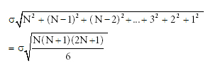
For comets Halley and Swift-Tuttle, these values are 130 years and 159 years, respectively.
Method B: Algebraic. For a particular comet:
t0: the Julian date for the oldest known perihelion
ti : an estimate of the Julian date for the ith unknown perihelion
P0: the oldest known period
Pi: an estimate for the ith unknown period
xi : the ith random variable from a [0, s] normal distribution of the changes in successive orbital periods of a comet
t1 = t0 - P0 + x1 P1 = t0-t1 = P0-x1
t2 = t1 - P1+ x2 = (t0 - P0+ x1) - (P0- x1) + x2 = t0 - 2P0 + 2x1 + x2 P2 = t1-t2 = P1-x2 = (P0-x1) - x2 = P0-x1 - x2
t3 = t2 - P2+ x3 = (t0 - 2P0 + 2x1 + x2) - (P0-x1 - x2) +x3 = t0 - 3P0 + 3x1 +2x2 + x3 P3 = t2-t3 = P2-x3 = (P0-x1 - x2) - x3 = P0-x1 - x2 -x3
...
tN = t0 - NP0 + Nx1 + (N-1)x2 + (N-2)x3 + ... + 3xN-2 + 2xN-1 + xN
Methods A and B produce identical results and have probability distributions that depends on only s and N.
Method C: Simulation. Instead of working with the long summations in Method B, a computer can generate each xi as a random number from a [0, s] normal distribution and substitute them in the equations:
t1 = t0 - P0 + x1 P1 = t0 - t1
t2 = t1 - P1 + x2 P2 = t1 - t2
t3 = t2 - P2 + x3 P3 = t2 - t3
...
tN = tN-1 - PN-1+ xN
Each sequence of N random numbers (x1, x2, ..., xN ) will give one simulated date for the flood, which will, in general, differ from 3290 B.C. Thousands of those simulated dates will give us the error estimates for each comet individually (of 130 and 159 years) that were found exactly in Methods A and B. Adding the additional information that both comets formed at about the same time—based on the statistical significance of >99%—allows the combined error estimate for the date of the flood to be reduced to ± 100 years.
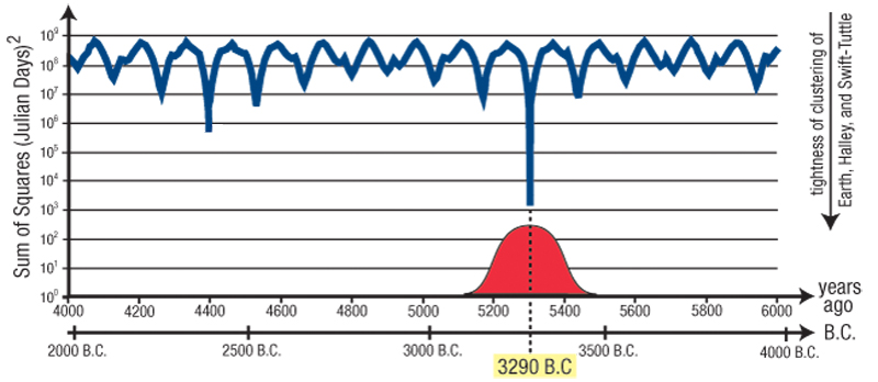
Figure 254: Comet Clustering. The tight clustering of comets Halley and Swift-Tuttle with Earth in 3290 B.C. (as shown above) does not mean that was the year of the flood. It simply means that 3290 B.C. is the most likely year of the flood, based on these calculations. As shown by the red normal distribution, the flood could have occurred within a hundred or so years of that date. The depth of this downward spike in 3290 B.C., however, is quite unusual. Had the backward projection of Halley and Swift-Tuttle started at a random point on their oldest known orbits instead of at their perihelions, it would take, on average, 333,333 years before a similar tightness of clustering of these three bodies (Earth and comets Halley and Swift-Tuttle) would be found. Is it merely a coincidence that we found a one-in-333,333-year event very near the time of the historical global flood—after a backward search of only 1290 years?
Also, basic physics tells us that gravitational perturbations are as likely to increase a comet’s period as to decrease a comet’s period; that is, a gravitational body, such as a planet, is as likely to pass in front of an orbiting comet at a certain distance as to pass behind it at that distance. While we may not know how the unknown periods changed, the statistical mean of those changes will be zero; therefore, the mean of the possible dates for the flood is 3290 B.C.
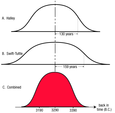
Figure 255: Probabilities for Perihelion Passage Dates. We have shown that if comets Halley and Swift-Tuttle had been projected back in time from their oldest known perihelions and with their oldest known periods, both comets would pass perihelion in the year 3290 B.C. Halley would have taken exactly 27 orbits and Swift-Tuttle exactly 22 orbits.
We also showed how unusual it is for both comets to be so close to Earth in any single year in the 2,000-year window in which almost all Bible scholars place the flood. Such a tight convergence would only happen 0.6 of 1% of the time. Nevertheless, the hydroplate theory explains why they were so close in the year of the flood.
Of course, each comet’s period would have changed slightly with each orbit, so while the year 3290 B.C. might be our best guess if we had to pick only one year for the comet’s simultaneous convergence with Earth, other years for the three-body convergence are also possible on either side of 3290 B.C. Projecting Halley back 27 orbits and allowing planetary perturbations similar to those seen with Halley’s most recent 45 orbits give us the distribution of possible years shown in Figure A above. Likewise, Figure B above gives the probability distribution of the possible years in which Swift-Tuttle passed perihelion on its 22nd orbit back in time from where we know it was on 702.30 B.C.
Finally, we have one other piece of information. Given that we are 99.4% confident that Halley and Swift-Tuttle were both near Earth in the same year, we will add the constraint to Figures A and B above that Halley made its 27th perihelion pass in the same year Swift-Tuttle made its 21st perihelion pass.
It can be shown, with some calculus and probability theory, that distribution C gives the probabilities—for each of the years on either side of 3290 B.C.—that both comets were simultaneously near Earth on a single year. That distribution has a standard deviation (sc ) of
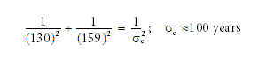
where Halley’s and Swift-Tuttle’s standard deviation in Figures A and B above were 130 years and 159 years, respectively.